3. Train from energy

This notebook walks you through training a normalizing flow by gradient descent when data is unavailable, but an energy function \(U(x)\) proportional to the density \(p(x)\) is available.

import matplotlib.pyplot as plt
import torch
import zuko

_ = torch.random.manual_seed(0)

3.1. Energy

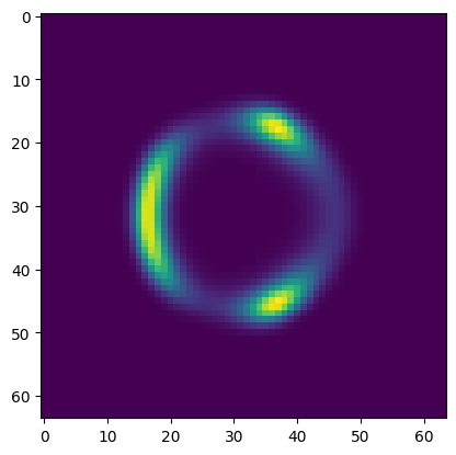
We consider a simple multi-modal energy function.

\[ \log U(x) = \sin(\pi x_1) - 2 \big( x_1^2 + x_2^2 - 2 \big)^2 \]

def log_energy(x):
    x1, x2 = x[..., 0], x[..., 1]
    return torch.sin(torch.pi * x1) - 2 * (x1**2 + x2**2 - 2) ** 2

x1 = torch.linspace(-3, 3, 64)
x2 = torch.linspace(-3, 3, 64)

x = torch.stack(torch.meshgrid(x1, x2, indexing="xy"), dim=-1)

energy = log_energy(x).exp()

plt.figure(figsize=(4.8, 4.8))
plt.imshow(energy)
plt.show()

3.2. Flow

We use a neural spline flow (NSF) as density estimator \(q_\phi(x)\). However, we invert the transformation(s), which makes sampling more efficient as the inverse call of an autoregressive transformation is \(D\) (where \(D\) is the number of features) times slower than its forward call.

flow = zuko.flows.NSF(features=2, transforms=3, hidden_features=(64, 64))
flow = zuko.flows.Flow(flow.transform.inv, flow.base)
flow

Flow(
  (transform): LazyInverse(
    (transform): LazyComposedTransform(
      (0): MaskedAutoregressiveTransform(
        (base): MonotonicRQSTransform(bins=8)
        (order): [0, 1]
        (hyper): MaskedMLP(
          (0): MaskedLinear(in_features=2, out_features=64, bias=True)
          (1): ReLU()
          (2): MaskedLinear(in_features=64, out_features=64, bias=True)
          (3): ReLU()
          (4): MaskedLinear(in_features=64, out_features=46, bias=True)
        )
      )
      (1): MaskedAutoregressiveTransform(
        (base): MonotonicRQSTransform(bins=8)
        (order): [1, 0]
        (hyper): MaskedMLP(
          (0): MaskedLinear(in_features=2, out_features=64, bias=True)
          (1): ReLU()
          (2): MaskedLinear(in_features=64, out_features=64, bias=True)
          (3): ReLU()
          (4): MaskedLinear(in_features=64, out_features=46, bias=True)
        )
      )
      (2): MaskedAutoregressiveTransform(
        (base): MonotonicRQSTransform(bins=8)
        (order): [0, 1]
        (hyper): MaskedMLP(
          (0): MaskedLinear(in_features=2, out_features=64, bias=True)
          (1): ReLU()
          (2): MaskedLinear(in_features=64, out_features=64, bias=True)
          (3): ReLU()
          (4): MaskedLinear(in_features=64, out_features=46, bias=True)
        )
      )
    )
  )
  (base): UnconditionalDistribution(DiagNormal(loc: torch.Size([2]), scale: torch.Size([2])))
)

The objective is to minimize the Kullback-Leibler (KL) divergence between the modeled distribution \(q_\phi(x)\) and the true data distribution \(p(x)\).

\[\begin{split} \begin{align} \arg \min_\phi & ~ \mathrm{KL} \big( q_\phi(x) || p(x) \big) \\ = \arg \min_\phi & ~ \mathbb{E}_{q_\phi(x)} \left[ \log \frac{q_\phi(x)}{p(x)} \right] \\ = \arg \min_\phi & ~ \mathbb{E}_{q_\phi(x)} \big[ \log q_\phi(x) - \log U(x) \big] \end{align} \end{split}\]

Note that this “reverse KL” objective is prone to mode collapses, especially for high-dimensional data.

optimizer = torch.optim.Adam(flow.parameters(), lr=1e-3)

for epoch in range(8):
    losses = []

    for _ in range(256):
        x, log_prob = flow().rsample_and_log_prob((256,))  # faster than rsample + log_prob

        loss = log_prob.mean() - log_energy(x).mean()
        loss.backward()

        optimizer.step()
        optimizer.zero_grad()

        losses.append(loss.detach())

    losses = torch.stack(losses)

    print(f"({epoch})", losses.mean().item(), "±", losses.std().item())

(0) -0.8076444268226624 ± 1.4574381113052368
(1) -1.5428426265716553 ± 0.1310734897851944
(2) -1.5719032287597656 ± 0.04953986406326294
(3) -1.5784311294555664 ± 0.022914621978998184
(4) -1.5850317478179932 ± 0.023105977103114128
(5) -1.5861082077026367 ± 0.022541742771863937
(6) -1.5803889036178589 ± 0.14612749218940735
(7) -1.5888274908065796 ± 0.017613010480999947

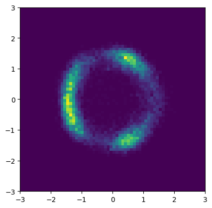
samples = flow().sample((16384,))

plt.figure(figsize=(4.8, 4.8))
plt.hist2d(*samples.T, bins=64, range=((-3, 3), (-3, 3)))
plt.show()